


Rurals of Nevada: Economic Well-Being Statistics - Part 1 (art. 14)
"The Economy of Well-Being . . . specifically highlights the need for putting people at the centre of policy." - OECD Secretary-General Angel Gurría, speech in Reykjavik, Iceland, 16 September 2019


On 14 February 2023, the Census Bureau released a new experimental data project known as the National Experimental WellBeing Statistics (NEWS). For some reason, the acronym makes me think this is, well, newsworthy.
The concept of “economic well-being” is emerging as an alternative measure of economic success in place of older measures such as Gross Domestic Product (GDP). In theory, the idea of developing an alternative to GDP accomplishes two tasks. First, it diminishes the importance of a single abstract variable that can only move in one direction—up or down. Second, it would allow a better look at how economic success (or failure) impacts society directly. Rather than just growing or shrinking, multiple axes can be used to get a more complete look at the entire economy in conjunction with the society of which it is part.
Unsurprising, this approach appeals to a number of critics of GDP-centric policy dynamics. These range from the Organization for Economic Co-Operation and Development (OECD) to advocates of non-growth sustainable economics such as Katherine Trebeck. In this openDemocracy article, Trebeck provides a good summary of what proponents believe a multi-parameter measure of economic well-being could achieve. As former OECD Secretary-General Angel Gurría noted in 2019, an idea of economic well-being is “moving away from an attitude of ‘grow first, redistribute and clean up later’, towards a growth model that is equitable and sustainable from the outset.”
But why the concept has a number of merits, there remains the issue of what exactly is going to be measured. A single figure such as GDP has the virtue of being easy to report and understand, even if we argue over how accurate the GDP of the U.S. or China might be in a given year. The U.S. Bureau of Economic Analysis (BEA) produces reports which calculate a GDP-per-capita measure to compare with the total GDP, as in its “Prototype Measures of Economic Well-Being and Growth” (most recent report here).
But they also are examining a range of other measures—which complicates what is meant by “economic well-being.” Any effort to develop a new measure are likely to be messy, but the problem with “well-being” is the range of items that are attempting to be incorporated. For instance, the OECD has been trying to develop a series of “well-being” measures since the 1970s. The result, their bi-annual How’s Life report, only appeared in 2011 (the most recent edition is from 2020, available here). The breadth of topics is impressive—but not necessarily clear to understand in toto. It is a lot of information.
While there is broad agreement that replacing GDP as a measure of “economic well-being” is needed, alternatives are complex and in flux. Two measures—median income and poverty levels—are playing a key role, however.
Two measures, however, emerge consistently as factors in determining economic well-being itself: median income and poverty levels. Taken together, these appear to give the best measure right now against the reliance on GDP. And that appears to be the working basis of the Census Bureau’s National Experimental WellBeing Statistics (NEWS) project. We can therefore look at these two measures together to see what they say about a basic concept of “economic well-being” in the Three Rurals we are discussing.
One vocabulary note: the Census Bureau and the NEWS project uses “WellBeing” but the term is more commonly rendered hyphenated as “Well-Being.” I will use the hyphenated form unless specifically referring to the NEWS paper.
National Experimental WellBeing Statistics (NEWS)
The report released on Valentine’s Day is an early effort of the Census Bureau to develop an economic well-being measure. The data release is concerned less with the results than assessing the accuracy of the statistics—which is frankly a very good approach. The resultant paper (Working Paper Number SEHSD WP2023-02; full paper here and executive summary and data here) was based on the 2019 Current Population Survey’s (CPS) Annual Social and Economic Supplement (ASEC), measuring 2018 income, and the 2018 American Community Survey (ACS). The analysis was conducted at a national level, broken down by demographic, household type, and income levels.
The goal was to assess the accuracy of the two measures by taking the data from the two Census Bureau surveys and comparing them to a range of other administrative data, ranging from the IRS and the Social Security Administration down to state agency data (SEHSD WP2023-02, pgs. 14ff). This reason accounts for the use of the 2018 data; it is likely the most recent all of these datasets contain. For an experimental project, this is not bad. It does miss the impact of the COVID-19 pandemic, but if the effort is to establish a baseline measure, that is not an issue.
Three issues were argued as seriously impacting the accuracy of the median income and poverty data:
Unit Nonresponse: A household not answering a survey at all
Item Nonresponse: Income information missing (a treasured American practice)
Misreporting: Errors in reporting income information
Generally, the first two errors (Unit and Item Nonresponse) tend to bias income up and poverty down, while misreporting tends to go the other way, dragging income down and poverty up (SEHSD WP2023-02, pgs. 5-6). The administrative data were used to assess and account for the impact of these issues on the measures.
The results were surprising. Overall, the adjusted median income was 6.3 percent higher than the survey estimates. The poverty level was 1.1 percentage points lower (equivalent to 9.4% fewer people in poverty). In other words, American households are wealthier on average than the official statistics show (SEHSD WP2023-02, pgs. 33ff). Moreover, the main issue is the misreporting of income, which is an interesting finding.
This underestimate of income was not consistent across all groups, however. There was a tendency for lower-income households to show a greater underestimation of income (meaning they were proportionally wealthier). Furthermore, Hispanic households showed slightly greater underestimation, particularly in the middle income percentiles, with little difference among other racial groups—although American Indians/Alaska Natives were not measured separately (SEHSD WP2023-02, pg. 59, Figure 7a). Region or metropolitan/non-metropolitan status did not show significant differences.
The NEWS-adjusted median income was up 6.3 percent and the poverty level was 1.1 percentage points lower. However, almost all of this difference was the result of changes to the reported wealth of a single age group, those 65 and older.
The single biggest factor, however, was age. Almost all the change in median household income and poverty level came from a single demographic group: the population 65 or older. This group had a median household income 27.3% higher than the surveys indicated, equivalent to almost $12,000 (2018 dollars). More astoundingly, the poverty rate for those 65 and older was 3.3 percent lower—equating to 34.1% fewer people in this age group in poverty. That was not a typo—34.1% fewer.
The graph below from the paper gives the income percent difference between the surveys and the experimental paper. Note that while the 55-64 age group also has slightly elevated discrepancies, all other age groups are in a very narrow band around the “no difference” line. There really is something different about the 65 and older age group when looking at this data.
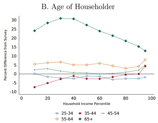
I also find it striking that difference is greater at lower and middle income percentiles but plunges in the upper percentiles. The NEWS paper does not speculate directly on the cause of the discrepancy uniquely with senior citizens, although the numerous comments on accounting for different types of taxable- and non-taxable income related to pension plans, disbursements, and Social Security payments provides a good sense of where the problems may lie.
These numbers are shocking and if accurate go against a long trend that has been tracking growing poverty among senior citizens. It is not surprising this is the takeaway of the report as identified by this Bloomberg article (behind a paywall—sorry) and will undoubtedly play the key message in other reporting over the next week.
But the finding also has a potentially major impact on one theme of this article series: the myth of the “Aging Rurals.” We have already examined the question of whether the Three Rurals really are aging in an earlier article. But the fact that this population might be wealthier adds a new wrinkle to the “aging tsunami”—if it holds. The NEWS report does not go into this level of geographic detail (that is something to be explored in future experimental papers), but we can dive into the original statistics to explore it.
Median Household Income in the Three Rurals
I will not attempt to duplicate the research of the NEWS paper—mainly because I have no access to the administrative data that would allow me to do so. However, since median household income and poverty level data are included in the ACS, we can get some idea of any differences between the Three Rurals and with the rest of the state.
And since I am not trying to replicate the NEWS study exactly, there is no reason to look at the 2018 data. I am going to use the 2021 ACS 5-Year Estimates, which cover the period from 2017 through 2021. This dataset is the most recent available and has the added bonus of covering before and the tail end of the COVID-19 pandemic. Remember, the 5-Year Estimates are not averages, but data calculated from five years of sampling. These, of course, have the usual problems of the ACS in terms of estimation bases and sampling issues, but I think they are good enough to establish patterns.
The main income data is contained in Table S1901: Income for the Last 12 Months. The Median Income figures are pre-tax and are given in four categories: Households, Families, Married-Couple Families, and Nonfamily Households. While the differences between these categories are important, the pattern of difference between them is relatively consistent (Married-Couple Families have higher median incomes than Families or Nonfamily Households, for instance). Therefore, I am only using the “Median Household Income” here to get a sense of an overall pattern.
The table below gives the median household incomes in the various regions of Nevada I am discussing, along with the United States for comparison. Since I do not have the individual responses for income, the median income column is an average of the county median incomes. It is a bit less precise, but can still give an idea of a pattern. Finally, I have added the percent population 65 or older from Table DP05.

Nevada’s median household income of $65,686 was over 95% of the national median household income, meaning for once we are not too far behind the rest of the nation. More surprising is there is not a sharp difference in median household income between the three urban counties and the 14 rural counties—only a 4.3% difference. If anything, the higher percentage of the population over 65 in the rurals might actually adjust this number closer to parity, if the NEWS data discussed above is correct. In either case, the close parallel in median household income between the urban and rural counties is actually a strong sign for Nevada’s economy.
Nevada’s median household income was close to the national median income and there is little difference between the three urban and fourteen rural counties collectively. Within the rural counties, however, there are sharp discrepancies.
But as usual, there are some sharp discrepancies between the Three Rurals. The Western Rural counties (Churchill, Douglas, Lyon, and Storey) have slightly higher median household incomes than the state median income (similar to the three urban counties, actually). Given the high percentage of senior citizens, this region might be even wealthier. And remember that Douglas County in particular, which has the third-highest median income in the state (after Lander and Elko Counties), is a “retirement destination” county attracting wealthier senior citizens.
It is the other two rural areas that are more divergent. The I-80 Corridor region is the wealthiest area in the state in terms of median household income, almost 115% of the state median. Four of the five counties (Elko, Eureka, Humboldt, and Lander) have median incomes greater than the state average, and Pershing is at 95.7%. Furthermore, Lander, Elko, and Humboldt are among the five counties with the highest median income (the other two are Douglas and Washoe Counties). Undoubtedly, this reflects the high salary ranges in mining and in its associated professional services.
The story is reversed for the Central Rural counties, which are the least wealthy portion of the state. The average median household income of $50,600 is only 77% of the state median. Even given the relatively high percentage of the population 65 or older (27.3%) is not enough to compensate for this low income even if the NEWS adjustments are correct. Moreover, four of the five counties in the region (Esmeralda, Lincoln, Mineral, and Nye) are in the 5 lowest median income counties in the state (Churchill County was the other one). Even White Pine County, the wealthiest of the Central Rurals, has a median income below the state median at $63,590 (lower than Clark County). The Central Rurals are the poorest region of the state.
Poverty Levels in the Three Rurals
While median household income may tell us a lot about the wealth of an area, it does little to tell about a lack of economic well-being (unwell-being?). In this way, it is similar to the GDP metric which only changes along one axis (up or down) and says little about how that income is actually distributed. Income has to be placed in context.
Measures of poverty are one way to do so, although they are complex and subject to intense controversy. For instance, to what extent should noncash government subsidies (SNAP food stamps or housing subsidies) or capital gains be included? What about child tax credits? Likewise, how does one calculate poverty levels for institutional housing such as military barracks, long-term nursing home care, or even college dormitories? Currently, these groups are not included in the measure. And what does the poverty level mean—just the ability to purchase a baseline basket of groceries and housing, or should some minimum “standard of living” be included? It is questions such as this that the NEWS project is attempting to assess.
For the Census Bureau, however, the definitions used are those from the federal Office of Management and Budget (OMB). Similar to the race and ethnic categories I looked at in the last article, the OMB poverty standards are set forth in an official statistics policy, known as Statistical Policy Directive 14 (SDP 14). I am not interested in challenging the various aspects of this policy here, but the Census Bureau’s explanations of the various parameters used can be found here for anyone interested.
What I am going to do is look at the poverty levels as reported in the 2021 ACS 5-Year Estimates, the same survey used for the median household income discussion (apples to apples and all that). The table below, taken from Table S1701: Poverty Status in the Last 12 Months, gives some poverty statistics for the regions we are examining. The percentages are calculated from the numbers (they are not averages). The information is the number of people below the poverty line, both in the respective regions and for the two sub-groups: those Under 18 and those 65 and Older.

While the NEWS paper does not include an “Under 18” category (since they are not subject to household-level surveys), I am including them here because a key part of the argument against the “Aging Rurals” idea is the number of children around.
Once again, Nevada has a slightly higher percentage of its population under the poverty line than the nation as a whole—but not extremely so. Once again, Nevada is not an outlier. Moreover, a similar distribution of poverty occurs consistently: those 65 and older tend to have lower percentages in poverty than society as a whole, while those Under 18 tend to have a markedly higher percentage below the poverty line. Wealth is concentrated in the older demographics, and the NEWS experimental analytics would just increase this margin.
What is striking is the regional variations. While median household income was relatively even between the urban and rural counties collectively, poverty is less prevalent in the rurals—except for the population 65 and Older. The 14 rural counties contain just over 8% of Nevada’s population below the poverty line, less than their share of the state population. But slightly more rural senior citizens live in poverty. Given that the rural counties have a higher share of Nevada’s senior citizen population (13%) is high, this might not be too surprising.
The difference in poverty levels between urban and rural counties which have similar median household incomes problematizes the use of median income for economic well-being. The differences between the Three Rurals emphasize this problem.
The discrepancy between the urban and rural counties, however, indicates that median household income may be a questionable measure of economic well-being. The differences between the Three Rurals provide further complications. The Western Rural counties have the lowest percentage of those below the poverty line in the state; three are at 10% or less, and Storey County at 12% below the poverty line is still below the state level (except for the Under 18 population poverty, which is quite high). Combined with the high median household income levels, this might be the wealthiest area of Nevada.
Along the same lines, the Central Rural counties collectively have the highest poverty levels in the state, which tracks with the low levels of median household income. But the region has the county with the lowest poverty level in the state (Lincoln, with 5.6% of the population below the poverty line) as well as the highest (Mineral, at 19.6%). Both the median income and poverty levels indicate that this region is struggling economically in ways the rest of the state is not—but not evenly.
And then there is the I-80 Corridor. The region has the highest median income—but also has some of the higher poverty levels in the state, especially for the 65 and Older population. Of course, the area is not a “retirement destination” (blame the pogonip) and those senior citizens remaining are most likely those lacking the resources to move. But there is also a high level of child poverty as well—not as pronounced as in the urban counties, but not good.
I believe what is shown here is the distorting effect of the high mining and associated professional salaries. These salaries bump up the median household income—but the incomes for those not in these industries (or retired) drop precipitously. There are, in effect, more limited lower-middle-income opportunities. This is strong evidence for the impact of single industries on economics commonly associated with rural areas.
I will conclude with the real oddity: Eureka County. In terms of median household income, Eureka County is comfortably above the state median by roughly $2,300 per year. However, it has the second highest poverty level in the state at 18.3%, and strikingly high levels of Under 18 poverty (25.1%) and 65 and Older poverty (14.6%). It would be interesting to do more research here, but at the moment I am inclined to view this as the result of the inability of poverty levels to reflect some aspects of rural life. Eureka is a major ranching county, including a number of family ranches. Wealth, then, is often held more in land and any income is divided among larger families. Even with mining expanding, what these numbers may mean is an inability to capture a rural model of “economic well-being.”
Conclusions
The NEWS paper on experimental statistics raises a number of interesting issues and represents the complexity of trying to develop an easily-related measure of “economic well-being.” I look forward to seeing how this project develops. In particular, the breakdown of the adjustments along smaller geographical units would be most helpful. Do the same levels of wealth under-estimation exist in the rurals, where comparatively fewer people, especially those over 65, might be receiving public subsidies?
The public subsidies issue is at the heart of the economic well-being argument and illustrates why measuring income and poverty levels more precisely is needed. Expanded poverty relief is needed in rural areas, but traditional urban-oriented policies can often fail. Take, for instance, something like food stamps, which are one of the more successful poverty-relief programs. One issue of concern is their use in “food desert” areas that lack grocery stores or markets carrying nutritious, non-processed food. But a “food desert” situation in an urban area can be partially addressed by a matching public transit subsidy. A rural “food desert” situation might mean an hour or longer drive to a grocery store where no public transit is available, drastically increasing the cost to “use” the relief. The cost here is not captured by either the income or poverty statistics.
Moreover, high median incomes in an area can work against poverty relief. The increased use of community block grant programs since the 1980s has helped drastically reduce poverty levels. But a basic requirement for many of these programs is defining a recipient group or area by income to qualify for the grants. In rural mining areas, median income levels make areas ineligible for many block grants even though they might have higher population percentages below poverty than winning urban areas. Solving this discrepancy will require re-thinking requirements.
For the next article, I want to try to break the data along slightly different lines than just county or regions. Thank you again for reading.